
B-pillar reinforcement: comparing a finished-part inventory with a process-level reconstruction
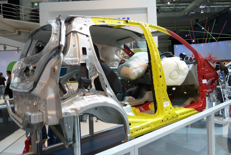
For a China-manufactured hot-stamped B-pillar reinforcement assembly at the same declared mass, this study compares a CALCD finished-component inventory with an eight-module ecoinvent-based reconstruction, examining material hotspots and the influence of manufacturing yields.
The same declared quantity, two inventory approaches
A representative engineering study, not an independently verified customer-product PCF or EPD. The baseline A−B difference is −0.477 kg CO₂-eq/assembly, or −5.31% relative to B; the ordering changes with material utilization, as discussed below.
Defining the quantity being compared
The reference assembly includes one hot-stamped main reinforcement, three cold-formed local plates and six M8 weld nuts, with a net mass of 1.818376 kg. Public part-mass information, a patented structural arrangement, standard nut masses and engineering assumptions define a traceable research scenario, rather than a confirmed complete design from a production vehicle.
The boundary includes steel and coating supply, blanking, hot stamping and quenching, trimming, local plates and fasteners, internal welding, utilities, inbound freight and production-scrap handover. Adjacent vehicle parts, whole-body e-coating, vehicle use and end of life are excluded. Crashworthiness, stiffness and fatigue equivalence were not verified, so the comparison uses the same declared quantity.
CALCD supplies the finished-component inventory in Configuration A
Configuration A scales the cumulative CALCD inventory for a left B-pillar reinforcement assembly once to 1.818376 kg. The record already includes its internal supply chain and manufacturing burdens, so steel, coating, nuts, welding, electricity and freight are not added again. The reference BOM defines the comparison mass; it does not disaggregate CALCD’s internal BOM.
Configuration B reconstructs eight foreground modules from public information and engineering parameters, linked to ecoinvent 3.12 cut-off backgrounds for China, Global and Rest-of-World regions. Purchased coil, furnace blanks, retained net mass and scrap are accounted for separately to test material utilization and process energy. Aggregation level, technology proxies and residual boundary differences all contribute to the comparison.
| Configuration B module | Activity |
|---|---|
| B10 / B20 | Main sheet supply; Al–Si coating |
| B30 / B40 | Laser blanking and trimming; hot forming and quenching |
| B50 / B60 | Local plates; M8 nut manufacture and delivery |
| B70 / B80 | Internal welding; scrap collection and handover |
Steel and coating dominate the reconstructed model
In Configuration B, main sheet supply, local reinforcement plates and Al–Si coating together account for 87.68% of climate impacts. This focuses data collection on steel production, gross-to-net material use and coating processes, rather than only electricity for final welding.
Source: report Table 6 and contribution analysis. Percentages use unrounded results; selected items do not sum to 100%. These module contributions apply only to B and cannot be projected onto A or directly used to explain the A/B difference.
| Configuration B contribution | kg CO₂-eq/assembly | Share of B |
|---|---|---|
| Main sheet supply | 5.320 | 59.20% |
| Local plates | 1.427 | 15.88% |
| Al–Si coating | 1.133 | 12.61% |
| Hot forming and quenching | 0.5008 | 5.57% |
| Laser blanking and trimming | 0.3880 | 4.32% |
One material-yield parameter can reverse the climate ordering
Baseline results are 8.510 kg CO₂-eq/assembly for A and 8.987 for B. Increasing B’s main-panel blanking utilization from 80% to 90% lowers B to 8.267 kg CO₂-eq/assembly, below the fixed A result. Finished assembly mass stays unchanged; gross material purchases and associated processes change to produce that same net mass.
The study tests low and high endpoints for 12 foreground parameters, giving 24 one-at-a-time runs. B ranges from 8.267 to 10.482 kg CO₂-eq/assembly. This demonstrates that engineering assumptions can change the baseline comparison; it is not a statistical confidence interval or proof of probabilistic superiority between databases.
| Main-panel blanking utilization | B climate result |
|---|---|
| 65% | 10.482 kg CO₂-eq/assembly |
| 80% (baseline) | 8.987 kg CO₂-eq/assembly |
| 90% | 8.267 kg CO₂-eq/assembly |
Interpret differences by indicator and modeling purpose
Across 16 primary EF categories, A is numerically lower than B in 12 and higher in four: human cancer toxicity, human non-cancer toxicity, freshwater ecotoxicity and marine eutrophication. The −5.31% climate difference therefore does not establish overall environmental superiority or an emissions reduction caused by acquiring data.
A finished-component inventory can connect directly to a purchase or product system when product and boundary match. Process-level reconstruction makes yield, process-energy and proxy choices more visible. The appropriate approach depends on the research question and available information. Equal mass and method do not turn this case into a single-variable test of database brand.
Conditions for applying the findings to another component
Reuse requires checking part geometry, steel grade, coating, gross inputs and net mass, yields, process energy and freight boundaries. The study retains limitations involving generic steel and fastener proxies, older European technology backgrounds and possible overlap between cold-rolling annealing and coating heat. CALCD’s internal BOM and plant parameters are not disclosed; B’s detail is not a decomposition of A.
The case shows how to compare two inventory approaches at an aligned declared quantity. Findings apply to this representative assembly and these model configurations. They cannot be linearly extrapolated to a whole-vehicle lifecycle or substitute for a customer component’s measured inventory and independent verification.
Choose the appropriate modeling level for your component
Share the part name, materials and manufacturing route, net mass, required boundary and available BOM. For a purchased-component estimate, begin by checking suitable finished-part records. For process optimization, add material yields, process energy and scrap information to determine which stages need explicit modeling.
Source: HiQLCD, Case study of a hot-stamped B-pillar reinforcement assembly: Modeling with HiQLCD and ecoinvent databases, version 1.0, 20 October 2026, supplied revised document; see Tables 5–7 and the appendix endpoint records.